 |
SLIMS |
 |
Inventory |
 |
Experiments |
|
|
SLIMS Database, supplemental
material for Chemistry and Biology
This database constitutes the
supplemental material for the Chemistry and Biology paper, Indoprofen
Upregulates The Survival Motor Neuron (SMN) Protein Through a
Cyclooxeganse Independent Mechanism
This database contains all of the screening data and analyses used to
generate the results in this paper.
To use, first install SLIMS from http://slims.sourceforge.net/
You may wish to install Java 1.4 from Sun in order to substructure
search the dataset. Java can be downloaded from http://www.java.com/
In this tutorial you will learn how to:
1) Navigate to the results section
2) Open up projects and their related
experiments.
3) View dilution series results.
4) View primary
screen results
5) Make a Self-Organiging Map
6) Peform a Medline Analysis
Here is a brief walkthrough of the dataset:
Navigate
to the Results Set
The initial screen that will open is the main database screen.
You will not have to log into this database, you will automatically be
logged in as administrator.
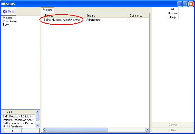
To view results, navigate to the results
section by clicking on the
results item in the navigation pane.
You will see the following window:
The results section is comprised of
Projects, each of which may have several experiments. There is
only one project in this database, namely the SMA project. To see
the project experiments, either double click on the project or select
the project and then select the experiments tab.
Viewing
Dilution Series
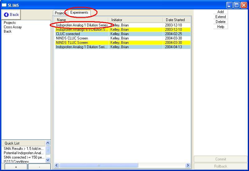
We will start off by selecting the Indoprofen Analog dilution series as
shown below:
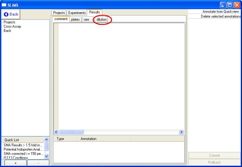
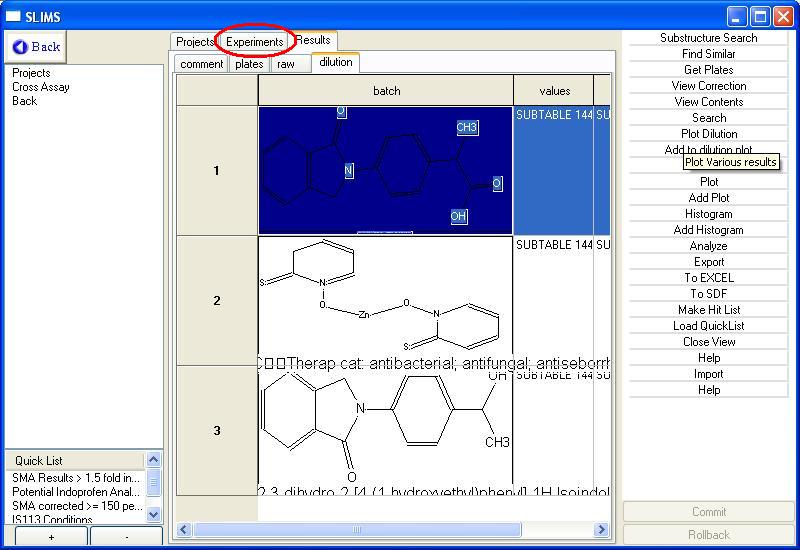
Naturally, we would like to see the dilution series. Click on the
dilution tab:
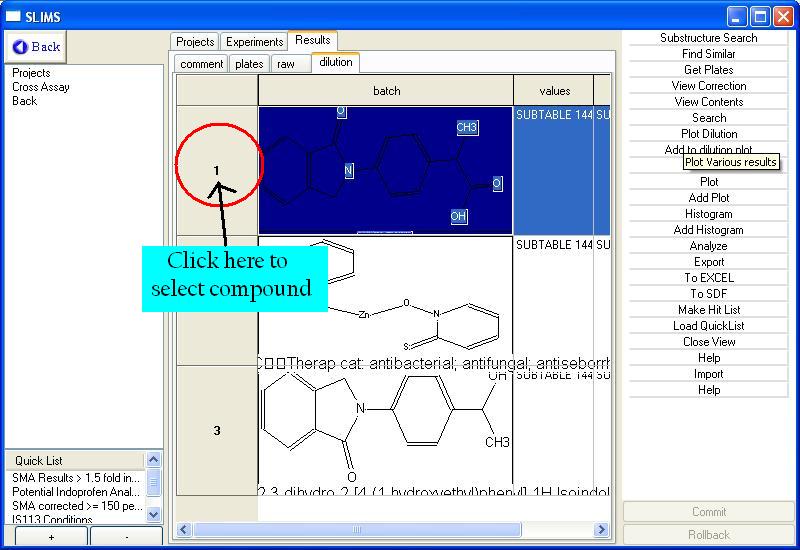
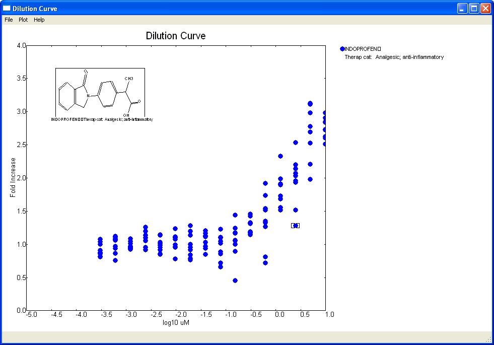
You will now see a collection of compounds, all of which contain
dilution series. To view a dilution series, select the compound
of interest and then click on the Plot
Dilution button from the commands
menu. For most selection criteria such as compound selection, you
must select the desired row. To select a row, click on the row
label as shown in the image:

You will then see the following graph:

If you would like to make a Microsoft Excel report for the dilution
series (and Microsoft Excel is installed in your system) , simply click
on the To Excel button. You will get a worksheet organized as
follows:
| Batch
ID |
Vendor |
Catalogue Number |
Name |
|
|
|
|
|
|
|
|
|
|
|
| 5382 |
NINDS |
1500351 |
INDOPROFEN
Therap cat: Analgesic; anti-inflammatory |
|
|
|
|
|
|
|
|
|
|
|
|
|
Average |
Standard Deviation |
Concentration |
Unit |
Values |
|
|
|
|
|
|
|
|
|
|
0.913909 |
0.098091815 |
0.000305 |
uM |
1.071891 |
0.858663 |
0.813809 |
1.036725 |
0.810129 |
0.905925 |
1.001003 |
0.877012 |
0.850027 |
|
|
0.994117 |
0.125856267 |
0.00061 |
uM |
0.751704 |
1.120885 |
0.964472 |
1.082781 |
1.058371 |
0.940237 |
0.857238 |
1.103127 |
1.068233 |
|
|
0.975944 |
0.057272039 |
0.001221 |
uM |
1.082242 |
0.929279 |
1.013926 |
0.931256 |
0.924118 |
0.948988 |
0.96355 |
0.94494 |
1.045203 |
|
|
1.063237 |
0.121272047 |
0.002441 |
uM |
0.914557 |
1.193801 |
1.053489 |
1.051002 |
0.954975 |
1.098901 |
1.257361 |
1.132671 |
0.912372 |
|
|
0.98509 |
0.107714542 |
0.004883 |
uM |
1.142967 |
1.006335 |
0.913637 |
0.851119 |
0.953363 |
0.847895 |
1.03078 |
0.984719 |
1.134998 |
|
|
1.032169 |
0.130544906 |
0.009766 |
uM |
1.099953 |
1.073501 |
0.987704 |
1.236839 |
0.953133 |
0.960272 |
1.092892 |
1.108478 |
0.776749 |
|
|
0.9839 |
0.182872352 |
0.019531 |
uM |
0.952281 |
1.275918 |
0.915477 |
1.197231 |
1.131371 |
0.759467 |
0.994722 |
0.840024 |
0.788613 |
|
|
1.038596 |
0.118107293 |
0.039063 |
uM |
1.161138 |
0.849002 |
1.124795 |
1.030738 |
1.199994 |
0.933789 |
1.114526 |
0.966807 |
0.966574 |
|
|
0.954293 |
0.188731997 |
0.078125 |
uM |
1.014386 |
0.882125 |
0.656246 |
1.039488 |
1.222792 |
0.718246 |
1.099405 |
1.100568 |
0.855377 |
|
|
1.051995 |
0.274185854 |
0.15625 |
uM |
0.452218 |
1.162518 |
1.047509 |
0.895102 |
1.241905 |
0.997577 |
1.171753 |
1.05823 |
1.441138 |
|
|
1.260496 |
0.11891338 |
0.3125 |
uM |
1.173789 |
1.162288 |
1.327902 |
1.187329 |
1.451922 |
1.170518 |
1.306911 |
1.143605 |
1.420201 |
|
|
1.352682 |
0.39262458 |
0.625 |
uM |
1.263957 |
1.736647 |
0.807138 |
1.512716 |
1.348065 |
1.91778 |
1.327615 |
1.539772 |
0.720452 |
|
|
1.793127 |
0.263609834 |
1.25 |
uM |
1.512608 |
1.728596 |
1.907321 |
1.896364 |
1.550021 |
2.326989 |
1.678885 |
1.555358 |
1.982 |
|
|
1.960254 |
0.371294419 |
2.5 |
uM |
2.069485 |
1.951255 |
2.199906 |
2.534473 |
1.275757 |
2.028315 |
2.134838 |
1.513718 |
1.934544 |
|
|
2.707835 |
0.402670015 |
5 |
uM |
1.980698 |
3.107103 |
2.523313 |
2.692676 |
2.981218 |
3.12215 |
2.208116 |
2.775266 |
2.979979 |
|
|
2.748159 |
0.152760948 |
10 |
uM |
2.6006 |
2.975992 |
2.83384 |
2.726066 |
2.621058 |
2.90085 |
2.724087 |
2.840634 |
2.510301 |
Viewing Primary Screening
Results
Go back to the experiments section by clicking on the Experiments
tab.

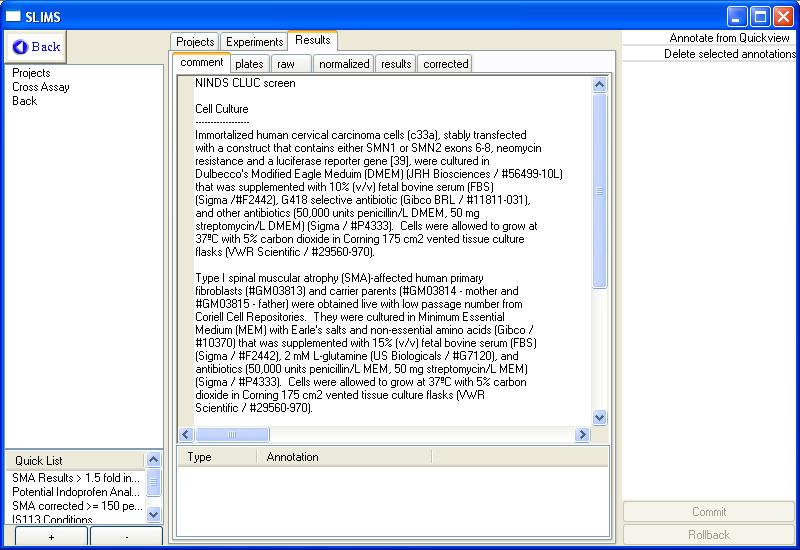
Double click on the NINDS CLUC Screen to view the primary screening
results of the NINDS CLUC screening
data. NINDS is a collection
of bioactive compounds obtained from the National Institute of Neurological
Disorders and Stroke. The initial screen shows related
comments, in this case it is the cell culture and compound seeding
methods used to prepare the screen.

Notice the six tabs at the top of the
screen.
Tab
|
Description
|
comment
|
This tab contains comments about
the experiment. This is a good place to place cell culture
descriptions and various assay related information.
|
plates
|
This tab shows a view of all the
plates used in the dataset. These plates also show the detected
systematic error. Any value below 0.05 is considered suspect and
should be analyzed by hand.
If the dataset has been corrected, this view also shows the plates that
have had systematic error removed.
|
raw
|
This tab shows the raw data
collected from each plate as well as the scored data. This is a
global view of the experiment and does not show any replicate statistic
data. The control wells are also present in this view.
|
normalized
|
If the data set has been loaded
with the option to correct systematic error, this tab shows the raw
data from each plate after the systematic error has been
normalized. Similar to the raw data, this tab does not show
replicate data. The control wells are also present in this view.
|
results
|
This tab shows the results
organized by replicates. For each batch (compound) in the
dataset, this view sumarizes all the replicate data including the
average and standard deviation of both the raw data and the scored
data. For instance, if the protocol was computing percent
enhancement, this view shows the statistics for the percent enhancement
for all batches (compounds) in the screen.
|
corrected
|
This
is the same as the results tab except that it computes the score (i.e.
percent enhancement) and raw data from the systematic error corrected
plates.
|
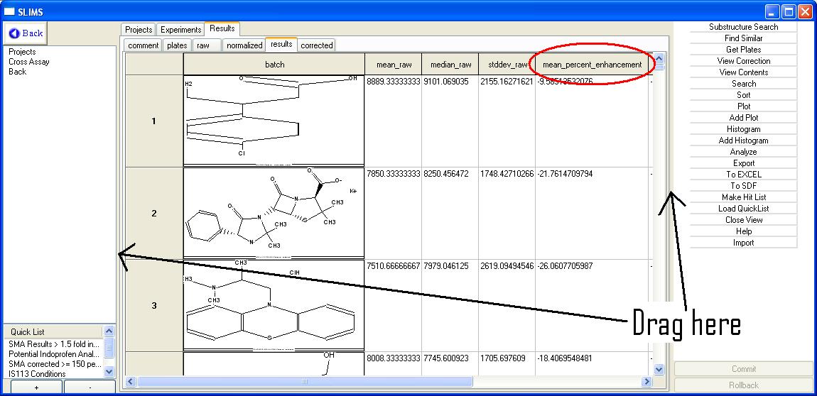
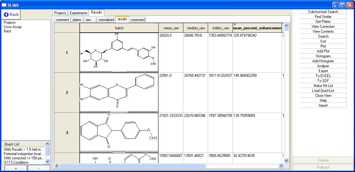
Select the results data tab. At
this point you may want to make the scren larger to view more
data. Note that to the left
and right of the data view there are sashes that you can drag to the
left and right to increase the size of the viewed data. See the
image below. Clicking on any header in the grid will sort
the data in that column. The first click will sort descending,
the second will sort ascending and the third will revert to the
original view. Click on the mean_percent_enhancement tab.
After sorting the data, the view will look like this:
Now the data is sorted by the top compounds. You might want to
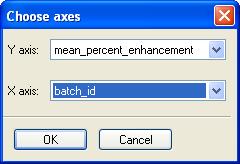
plot the data as well. Click on the plot button in the commands
menu. Select "mean_percent_enhancement" for the Y axis and
"batch_id" for the X.

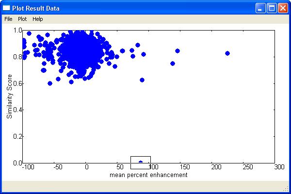
Click ok. You will see the
following plot:

Click on a point in the plot will
highlight the structure in the view window. The box shown
highlighted above is our friend Indoprofen which is one of the top hits
from the NINDS dataset. To see if there are any similar compounds
to indoprofen, click on Find Similar in the commands menu. This
will compute a similarity score based on the compounds fingerprint and
rank all compounds relative to the selected structure. A
Similarity score of 0 indicates that there is no difference in
fingerprint while a score of 1 means that the fingerprints have nothing
in common. note: this is normally called a diference
score.
Now from the newly
created Similarituy view, make a new plot, this time with Similarity
Score as the Y axis and mean percent enhancement as the X axis.
You
will see the following plot.

The
highlighted compound at the bottom (at Similarity score 0) is
indoprofen. Note that this compound stands alone. There are
no compounds clustered near this data point indicating that the
structure of indoprofen is highly different than any other structure in
the NINDS data set.
Making
a SOM
Final,
we will make a self-organizing map in order to
browse through the dataset. A self organizing map is an analysis
technique that is used to place similar compounds together in
space. The SOM is a collection of connecting nodes where nodes
closer together are generally more similar than nodes farther apart.
To create a SOM, click on the analyze button in the commands
pane. You have two options at this point, View Self Organizing
map or Create self organizing map. Viewing an existing map will
allow you to plate compounds located in a quicklist.
This is useful if you have already created a SOM and wish to see where
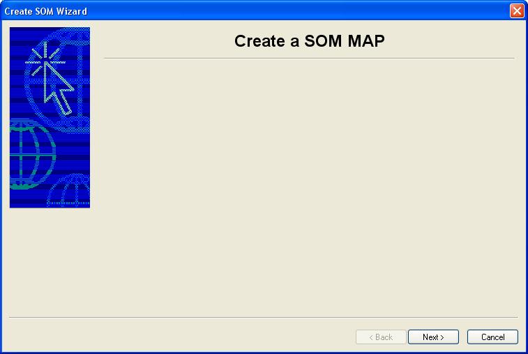
new compounds fall. Click on Create
Self Organizing Map. You will see a wizard at this point.

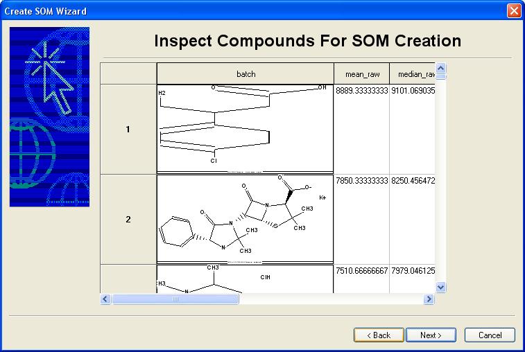
Clicking on Next will show you the
current compound set that you are going to use to create the SOM.

Note that the SOM only uses the
compounds fingerprint to generate the data. Click on Next to set
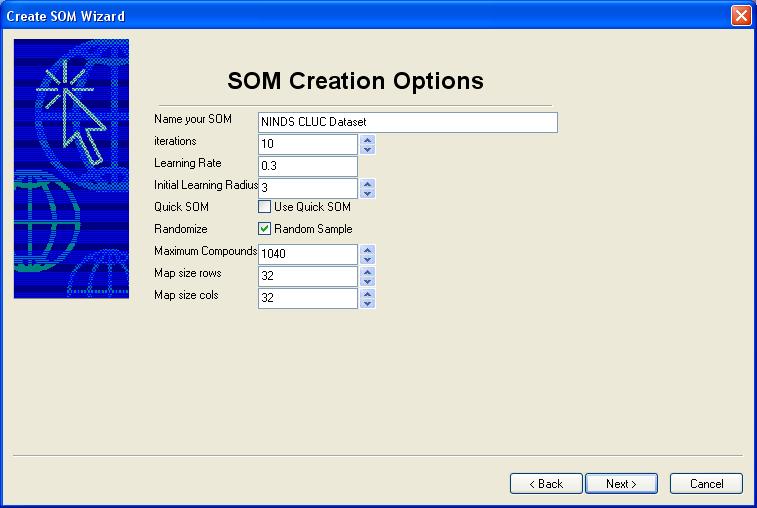
the creation options.

In general, the default values are
appropriate to use. Remember that the size of the map (Map size
rows and Map size cols) above, the number of iterations and the number
of compounds will influence the time it takes to generate a self
organizing map. Once the map has been started, you will not be
able to stop the operatation until the generation of the map has
completed. You may click on Quick SOM to make the map faster at
the expense of quality, although this might be appropriate for browsing.
Enter a name for the SOM such as NINDS CLUC Dataset and click on
next. This map will take about five to ten minutes to build on a
current computer (1.5gHz to 2.0gHz PC).
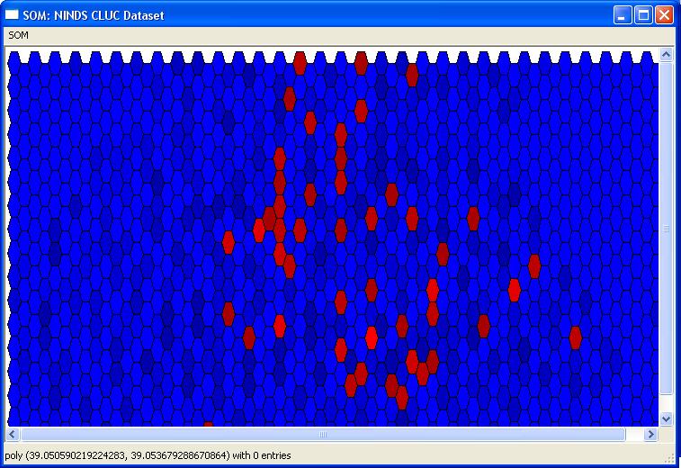
When the SOM is complete, click on finish and the SOM will appear
(Note, due to the random nature of SOM generation, the map you see will
look not look exactly as follows) You can resize the window if it
is too small. The map is initially colored by the number of
compounds in a node. Red has the most and dark blue has the
least. Holding the cursor over a node will indicate how many
compounds are in a well.

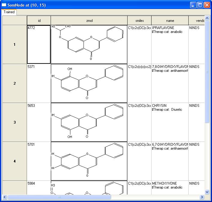
Clicking on a well will show the
compounds in the well, for example this node has compounds with a
Dihydroxyflavone motif:

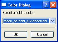
The som can also be recolored based on
various data. Click on the SOM menu and then click on
recolor. Choose mean_percent_enhancement

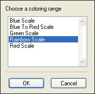
Then choose your favorite coloring
scheme:

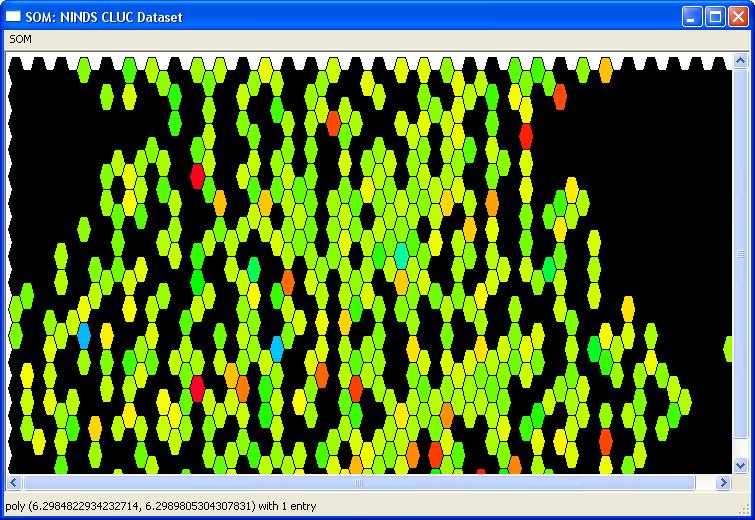
The map will then be recolored using the
selected criteria:

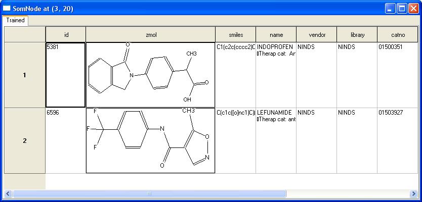
Clicking on the light blue hits (purple,
indigo...) wil reveal clusters of higher scoring compounds. We
immediately find indoprofen using this technique:

Note that, in general, this is not a
good way to find singlular hits, but is intended to find clusters of
hits with similar structures.
Perform A Medline Analysis
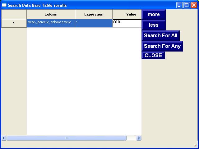
Now, go back to the results tab and click on search and find all
compounds that have greater than 60% percent enhancement:

Set the column to
"Mean_percent_enhancement" and the expression to ">" then set the
value to 60. Click on Search
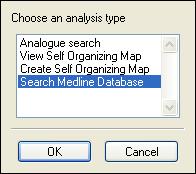
for All. Inspect the newly created Search tab and then
click on Analyze and select Search Medline Database.

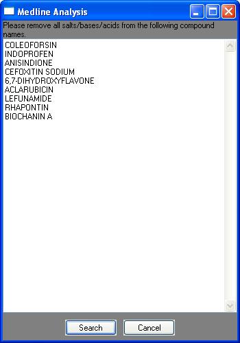
You will be presented with a list of
drug names. These only appear if your selected drugs actually do
have names, if they do not, then you cannot search medline.
Obviously, if the drug name is novel and does not appear in Medline,
you will not find any results either.

The next step is to remove all
salts/base and acids identifiers from the drug names as well as any
extraneous information. Simply edit the text in the window and
click on Search.
You will be presented with the Medline Search result seen below.
Each mechanism link takes you to the relevant papers in PubMed.
Notice that there is at least on Cyclooxegenase result from the
Indoprofen compound. This table is a good way to organize
mechanisms with hit compounds. Unfortunately, you need to screen
compounds such as the Active Compound Library for maximum effectiveness
when using the Medline Searching Capabillity. The index Medline
papers only go through 2002, we are in the process of indexing 2003 and
will release the index when it is available.
Medline Analysis
Medline Annotation v 1.0
| mechanism |
literature percentile |
compound percentile |
score |
%hits |
%drugs |
num selected drugs |
num Library drugs |
num selected papers |
num Library papers |
selected mean |
selected median |
selected std |
Library mean |
Library median |
Library std |
pos |
neg |
epos |
eneg |
drug |
drug |
| ANTIBIOTICS |
3.00E-001 |
3.00E-001 |
9.00E-002 |
0.1111 |
0.0602 |
1 |
177 |
1 |
194 |
1.0000 |
1.0000 |
NAN |
1.5763 |
1.5763 |
NAN |
1 |
176 |
0.5418 |
176.4582 |
ACLARUBICIN |
| ANTIOXIDANTS |
3.00E-001 |
3.00E-001 |
9.00E-002 |
0.1111 |
0.0231 |
1 |
73 |
1 |
66 |
1.0000 |
1.0000 |
NAN |
1.4795 |
1.4795 |
NAN |
1 |
67 |
0.2082 |
67.7918 |
ACLARUBICIN |
| PROTEIN
SYNTHESIS |
4.00E-001 |
4.00E-001 |
1.60E-001 |
0.1111 |
0.0143 |
1 |
42 |
1 |
39 |
1.0000 |
1.0000 |
NAN |
1.3095 |
1.3095 |
NAN |
1 |
41 |
0.1286 |
41.8714 |
ACLARUBICIN |
| DNA |
5.00E-001 |
5.00E-001 |
2.50E-001 |
0.1111 |
0.1167 |
1 |
359 |
1 |
659 |
1.0000 |
1.0000 |
NAN |
2.6657 |
2.6657 |
NAN |
1 |
342 |
1.0500 |
341.9500 |
ACLARUBICIN |
| GLYCOSYLATION |
5.00E-001 |
5.00E-001 |
2.50E-001 |
0.1111 |
0.0082 |
1 |
25 |
1 |
25 |
1.0000 |
1.0000 |
NAN |
1.3200 |
1.3200 |
NAN |
1 |
23 |
0.0735 |
23.9265 |
ACLARUBICIN |
| UP |
5.00E-001 |
5.00E-001 |
2.50E-001 |
0.1111 |
0.0898 |
1 |
281 |
1 |
267 |
1.0000 |
1.0000 |
NAN |
1.4270 |
1.4270 |
NAN |
1 |
263 |
0.8082 |
263.1918 |
RHAPONTIN |
| ANTI-INFLAMMATORY
AGENTS |
5.00E-001 |
5.00E-001 |
2.50E-001 |
0.1111 |
0.0412 |
1 |
129 |
1 |
135 |
1.0000 |
1.0000 |
NAN |
1.6744 |
1.6744 |
NAN |
1 |
120 |
0.3704 |
120.6296 |
INDOPROFEN |
| PHOSPHATASE |
5.00E-001 |
5.00E-001 |
2.50E-001 |
0.1111 |
0.0231 |
1 |
74 |
1 |
56 |
1.0000 |
1.0000 |
NAN |
1.4324 |
1.4324 |
NAN |
1 |
67 |
0.2082 |
67.7918 |
RHAPONTIN |
| ANTIBIOTIC |
5.00E-001 |
5.00E-001 |
2.50E-001 |
0.1111 |
0.0316 |
1 |
93 |
1 |
91 |
1.0000 |
1.0000 |
NAN |
1.4839 |
1.4839 |
NAN |
1 |
92 |
0.2847 |
92.7153 |
ACLARUBICIN |
| CDK2 |
5.00E-001 |
5.00E-001 |
2.50E-001 |
0.1111 |
0.0041 |
1 |
12 |
1 |
9 |
1.0000 |
1.0000 |
NAN |
1.3333 |
1.3333 |
NAN |
1 |
11 |
0.0367 |
11.9633 |
RHAPONTIN |
| JUN |
7.00E-001 |
7.00E-001 |
4.90E-001 |
0.1111 |
0.0932 |
1 |
287 |
1 |
410 |
1.0000 |
1.0000 |
NAN |
1.6481 |
1.6481 |
NAN |
1 |
273 |
0.8388 |
273.1612 |
ANISINDIONE |
| CDK6 |
1 |
1 |
1 |
0.1111 |
0.0007 |
1 |
2 |
1 |
2 |
1.0000 |
1.0000 |
NAN |
1.0000 |
1.0000 |
NAN |
1 |
1 |
0.0061 |
1.9939 |
RHAPONTIN |
| ANTICOAGULANTS |
1 |
1 |
1 |
0.1111 |
0.0082 |
1 |
26 |
1 |
24 |
1.0000 |
1.0000 |
NAN |
1.4231 |
1.4231 |
NAN |
1 |
23 |
0.0735 |
23.9265 |
ANISINDIONE |
| CYCLOOXYGENASE |
1 |
1 |
1 |
0.2222 |
0.0221 |
2 |
69 |
2 |
59 |
1.0000 |
1.0000 |
0 |
1.4638 |
1.4638 |
1.5008 |
2 |
63 |
0.1990 |
64.8010 |
INDOPROFEN |
RHAPONTIN |
| CELL
CYCLE |
1 |
1 |
1 |
0.1111 |
0.0214 |
1 |
63 |
1 |
67 |
1.0000 |
1.0000 |
NAN |
2.0952 |
2.0952 |
NAN |
1 |
62 |
0.1929 |
62.8071 |
RHAPONTIN |
| TF |
1 |
1 |
1 |
0.1111 |
0.0058 |
1 |
18 |
1 |
16 |
1.0000 |
1.0000 |
NAN |
1.1111 |
1.1111 |
NAN |
1 |
16 |
0.0520 |
16.9480 |
ANISINDIONE |
| ANTICARCINOGENIC
AGENTS |
1 |
1 |
1 |
0.1111 |
0.0037 |
1 |
11 |
1 |
11 |
1.0000 |
1.0000 |
NAN |
1.0909 |
1.0909 |
NAN |
1 |
10 |
0.0337 |
10.9663 |
RHAPONTIN |
Missing Drugs
COLEOFORSIN
CEFOXITIN SODIUM
6,7-DIHYDROXYFLAVONE
LEFUNAMIDE
BIOCHANIN A
That is it for the introduction. Feel free to play with different
analyses and colorings.
|
